reticulate::py_install("saspy", pip = TRUE)Using SASPy
SASPy is an open-source Python package (maintained by the SAS Foundation) that behaves very similarly to how reticulate behaves. Just like reticulate is an R interface to Python, SASPy is a Python interface to SAS. By making use of both reticulate and SASPy, you can create R scripts that combine R, Python, and SAS code with interoperability between all languages.
You can find the full documentation for SASPy here.
Video instructions
If you prefer to learn by video, the tutorial below summarizes the information on this page.
Installing dependencies
In order to use SASPy, you’ll need to install the following: R, Python, SAS, and Java.
While there are many ways to install Python, you may wish to use reticulate::install_miniconda().
Next, install SASPy. If you’ve installed miniconda via the reticulate package, you can use
to install the package. To verify that the installation worked successfully, run
reticulate::py_module_available("saspy")and verify that the results return TRUE.
Performing system configurations
SASPy requires several system configurations in order to function properly. The instructions below are for a Windows machine and will allow you to run SAS locally from within your R scripts. For other configurations, refer to the SASPy documentation.
Step 1: Locating your configuration file
When you install SASPy, a configuration file called sascfg.py is created. The location of this file will depend on how you installed SASPy, but is most likely located in the site-packages folder in your Python installation. If you installed miniconda via reticulate, the sascfg.py file can likely be found in the following location: C:\Users\your-username-here\AppData\Local\r-miniconda\envs\r-reticulate\Lib\site-packages.
Step 2: Modifying the configuration file
Make a copy of the sascfg.py file in the same folder, and rename the copy of the file to sascfg_personal.py.
Open up the sascfg_personal.py file in a text editor and locate the part of the script that defines SAS_config_names. Switch which of the two SAS_config_names is commented out so that the line with just “default” has a hashtag in front of it, and the line with the longer list of names has no hashtag in front of it.
Step 3: Adding java as an environment variable
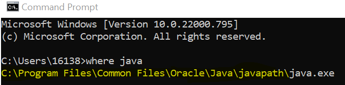
Open Command Prompt and type where java to determine the location of java on your machine. Copy the part up to but not including the java.exe to your clipboard.
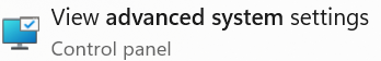
Go to Advanced System Settings on your computer.
Under “Advanced”, click “Environment Variables”.
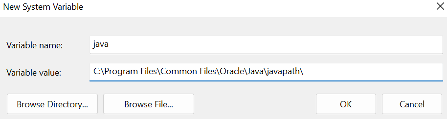
Click “New”. Name the variable java and set the variable path to the location of your java installation (copied to your clipboard from Command Prompt). Click OK.
Under “User variables”, highlight “Path” and then click “Edit”.
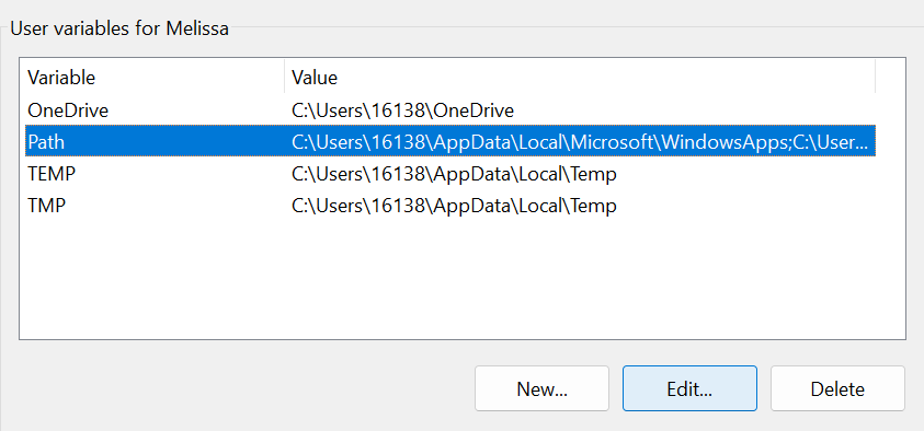
Click “New”. Type %java%\bin and hit Enter, then click OK until all Control Panel windows are closed.
How to use SASPy
You’re now ready to begin using SASPy! First, you’ll need to load the reticulate package and import saspy.
library(reticulate)
saspy <- import("saspy")
Next, create a SAS session and assign it to a variable. Here, we’re using the “Windows local” configuration, but other configuration options are described in the SASPy documentation.
sas_sess <- saspy$SASsession(cfgname = "winlocal")If everything was configured correctly, you should see a message in the console indicating that the connection was successfully established.

Let’s walk through an example analysis that combines R, Python, and SAS in the same script.
First, let’s make the penguins dataset from the palmerpenguins package visible to SAS. We do this using the dataframe2sasdata function that’s accessible through the sas_sess object.
library(palmerpenguins)
sas_sess$dataframe2sasdata(df = penguins,
                           table = "sas_penguins")
We can now apply SAS code directly to this R data frame. To do this, we use the submit function, again accessible through the sas_sess object. In this example, we’re using the frequency procedure in SAS (proc freq) to create a frequency table of the species and islands variables from the penguins dataset.
submit_sas <- sas_sess$submit("proc freq data=sas_penguins; tables species * island / out=work.my_results; run;")We can bring the results back into R using sasdata2dataframe.
penguins_freqs <- sas_sess$sasdata2dataframe("my_results")
penguins_freqs| species | island | COUNT | PERCENT |
|---|---|---|---|
| Adelie | Biscoe | 44 | 12.79070 |
| Adelie | Dream | 56 | 16.27907 |
| Adelie | Torgersen | 52 | 15.11628 |
| Chinstrap | Dream | 68 | 19.76744 |
| Gentoo | Biscoe | 124 | 36.04651 |
We can also use pandas (from Python) to manipulate the R data frame by using reticulate.
# Import pandas (Python package) to be used in R
pd <- import("pandas", convert = FALSE)

# Convert penguins_freqs R data frame to a pandas DataFrame
penguins_freqs <- pd$DataFrame(data = penguins_freqs)

# Use pandas to drop the PERCENT column from penguins_freqs
penguins_freqs <- penguins_freqs$drop("PERCENT", axis = 1)
penguins_freqs| species | island | COUNT |
|---|---|---|
| Adelie | Biscoe | 44 |
| Adelie | Dream | 56 |
| Adelie | Torgersen | 52 |
| Chinstrap | Dream | 68 |
| Gentoo | Biscoe | 124 |